Introduction

The genome is the collection of an organism's DNA. All living beings have a genome, but the size of these can vary from one species to another. For example, the human genome has 23 chromosomes and each chromosome contains about 6 billion nitrogenous bases. Each human being has a unique genome of their own. However, the genome of two individuals only really differs by about 1%. The genomes of the same species are therefore actually very similar.

Machine Learning can be applied to genomics because of the very large amount of data exploited, the goal being to understand the links between the data to infer new hypotheses.

In our case, we will seek to predict the influence of genetic variation on gene regulation mechanisms, such as DNA receptivity and splicing in eukaryotic cells. In particular, we will understand how to interpret the structure of DNA so that its information is usable by Machine Learning algorithms in order to build a prediction model based on DNA sequences.

Representation of a DNA Sequence

DNA is a nucleotide made up of four types of nitrogenous bases: Adenine (A), Cytosine (C), Guanine (G), and Thymine (T). It is the hydrogen bonds that ensure the links between these chemical components by forming a chain.

DNA is most often represented by a double helix formed by two chains. Indeed, the second chain is obtained by complementarity with the first. If the first chain contains an A (resp. C), then in the second you will have a T (resp. G) by symmetry. Thus, by identifying one chain of the helix, we can deduce the second.

The sequence of DNA, i.e., the order of the nitrogenous bases, determines the biological information contained in a strand of DNA. For example, the sequence ATCGTT is the marker for blue eyes and ATCGCT for brown eyes.

Biopython Library: Computational Tools for Molecular Biology

from Bio import SeqIO

import matplotlib.pyplot as plt
import pandas as pd
import numpy as np
import os
import re

from sklearn.preprocessing import LabelEncoder
from sklearn.preprocessing import OneHotEncoder
from sklearn.feature_extraction.text import CountVectorizer
from sklearn.feature_extraction.text import CountVectorizer
from sklearn.model_selection import train_test_split
from sklearn.naive_bayes import MultinomialNB
from sklearn.metrics import accuracy_score, f1_score, precision_score, recall_score

# an example DNA sequence
for sequence in SeqIO.parse('data/dna-sequence-dataset/example_dna.fa', "fasta"):
    print("Sequence ID:", sequence.id)
    print("Sequence length:", len(sequence))
    print("-> [ {} ]".format(sequence.seq))
    break

Sequence ID: ENST00000435737.5
Sequence length: 390
-> [ ATGTTTCGCATCACCAACATTGAGTTTCTTCCCGAATACCGACAAAAGGAGTCCAGGGAATTTCTTTCAGTGTCACGGACTGTGCAGCAAGTGATAAACCTGGTTTATACAACATCTGCCTTCTCCAAATTTTATGAGCAGTCTGTTGTTGCAGATGTCAGCAACAACAAAGGCGGCCTCCTTGTCCACTTTTGGATTGTTTTTGTCATGCCACGTGCCAAAGGCCACATCTTCTGTGAAGACTGTGTTGCCGCCATCTTGAAGGACTCCATCCAGACAAGCATCATAAACCGGACCTCTGTGGGGAGCTTGCAGGGACTGGCTGTGGACATGGACTCTGTGGTACTAAATGAAGTCCTGGGGCTGACTCTCATTGTCTGGATTGACTGA ]

Encoding DNA Sequences

The data we have is in the form of character strings. To make them usable by a machine learning model, we need to encode them as matrices. There are several methods to do this:

Ordinal encoding

One-hot encoding

k-mer counting encoding

1) Ordinal Encoding

A value is associated with each nitrogenous base.

def string_to_array(sequence):
    sequence = sequence.lower()
    sequence = re.sub('[^acgt]', '', sequence)
    sequence = np.array(list(sequence))
    return sequence

# create a label encoder with the alphabet {a,c,g,t}
label_encoder = LabelEncoder()
label_encoder.fit(np.array(['a', 'c', 'g', 't']))

def ordinal_encode(array):
    integer_encoded = label_encoder.transform(array)
    float_encoded = integer_encoded.astype(float)
    float_encoded[float_encoded == 0] = 0.25  # A
    float_encoded[float_encoded == 1] = 0.50  # C
    float_encoded[float_encoded == 2] = 0.75  # G
    float_encoded[float_encoded == 3] = 1.00  # T
    float_encoded[float_encoded == 4] = 0.00  # any other letter
    return float_encoded

# test the program on a short sequence:
test_sequence = 'TTCAGCCAGTG'
ordinal_encode(string_to_array(test_sequence))

array([1.  , 1.  , 0.5 , 0.25, 0.75, 0.5 , 0.5 , 0.25, 0.75, 1.  , 0.75])

2) One-Hot Encoding

One-hot encoding represents each state of a variable with n states using n bits, where only one bit is set to 1, corresponding to the number of the state taken by the variable. Thus, "ATGC" becomes [0,0,0,1], [0,0,1,0], [0,1,0,0], [1,0,0,0], and we can then concatenate the vectors or transform them into two-dimensional arrays.

def one_hot_encode(string):
    integer_encoded = label_encoder.transform(string)
    onehot_encoder = OneHotEncoder(sparse=False, dtype=int)
    integer_encoded = integer_encoded.reshape(len(integer_encoded), 1)
    onehot_encoded = onehot_encoder.fit_transform(integer_encoded)
    onehot_encoded = np.delete(onehot_encoded, -1, 1)
    return onehot_encoded

# test the program on a short sequence:
test_sequence = 'GAATTCTCGAA'
one_hot_encode(string_to_array(test_sequence))

array([[0, 0, 1],
       [1, 0, 0],
       [1, 0, 0],
       [0, 0, 0],
       [0, 0, 0],
       [0, 1, 0],
       [0, 0, 0],
       [0, 1, 0],
       [0, 0, 1],
       [1, 0, 0],
       [1, 0, 0]])

3) k-mer Counting Encoding

None of the previous methods directly provide a vector of uniform length (required for machine learning algorithms). Let's view the genome as a book: genes are sentences, sequences of amino acids are words, and nucleotides and bases form the alphabet. Following this analogy, we will implement an NLP (natural language processing) algorithm called "k-mer counting". Thus, we take a long biological sequence and divide it into k-mers (strings of length k). For example, if k=6, then "ATGCATGCA" is divided into four 6-mers (hexamers): "ATGCAT", "TGCATG", "GCATGC", "CATGCA".

def kmers(sequence, k):
    return [sequence[index:index+k].upper() for index in range(len(sequence) - k + 1)]

# test the program on a short sequence:
test_sequence = 'ATGCATGCA'
kmers(test_sequence, 5)

['ATGCA', 'TGCAT', 'GCATG', 'CATGC', 'ATGCA']

The k-mers can then be concatenated into a sentence:

words = kmers(test_sequence, 5)
sentence = ' '.join(words)
sentence

'ATGCA TGCAT GCATG CATGC ATGCA'

You can tune both the word length and the amount of overlap. This allows you to determine how the DNA sequence information and vocabulary size will be important in your application. For example, if you use words of length 6, and there are 4 letters, you have a vocabulary of size 4096 possible words. You can then go on and create a bag-of-words model like you would in NLP.

Let’s make a couple more “sentences” to make it more interesting.

sequence1 = 'TCTCACACATGTGCCAATCACTGTCACCC'
sequence2 = 'GTGCCCAGGTTCAGTGAGTGACACAGGCAG'
phrase1 = ' '.join(kmers(sequence1, 6))
phrase2 = ' '.join(kmers(sequence2, 6))

# Next, we build the bag-of-words model
cv = CountVectorizer()
X = cv.fit_transform([phrase, phrase1, phrase2]).toarray()
X

array([[0, 0, 0, 0, 0, 0, 0, 0, 0, 0, 0, 2, 0, 0, 0, 0, 0, 0, 0, 0, 0, 1, 0, 0, 0, 0, 
	   0, 0, 0, 0, 1, 0, 0, 0, 0, 0, 0, 0, 0, 0, 0, 0, 0, 0, 0, 0, 0, 1, 0, 0, 0, 0, 0],
       [1, 0, 1, 0, 1, 1, 0, 0, 0, 0, 1, 0, 1, 1, 1, 0, 1, 1, 0, 0, 0, 0, 1, 1, 0, 0, 
	   1, 1, 0, 0, 0, 1, 0, 0, 1, 0, 0, 1, 0, 0, 1, 1, 1, 0, 1, 0, 0, 0, 1, 0, 1, 1, 0],
       [0, 1, 0, 1, 0, 0, 1, 1, 1, 1, 0, 0, 0, 0, 0, 1, 0, 0, 1, 1, 1, 0, 0, 0, 1, 1, 
	   0, 0, 1, 1, 0, 0, 1, 1, 0, 1, 1, 0, 1, 1, 0, 0, 0, 1, 0, 1, 1, 0, 0, 1, 0, 0, 1]], 
	   dtype=int64)

Project Context and Objectives

Now that we know how to extract a matrix containing the information from a DNA sequence, we can use this data and apply it in the context of Machine Learning.

Our objective is to build a classification model that takes human DNA sequences as training data and can predict the "family" to which a particular gene belongs. Unlike the training data, the test data will be more diverse, and the DNA can come from a human, a dog, or a chimpanzee. We can then study the consequences of this genetic diversification on the performance of the model.

The "family" of a gene is a group of related genes that share a common ancestor. Two genes in the same family can be paralogs or orthologs. Paralogous genes have similar sequences within the same species, while orthologous genes have similar sequences across different species.

Loading DNA Sequences

Human DNA

human_dna = pd.read_table('data/dna-sequence-dataset/human.txt')
human_dna.head()

	-------------------- sequence ------------------- class
0	ATGCCCCAACTAAATACTACCGTATGGCCCACCATAATTACCCCCA...	4
1	ATGAACGAAAATCTGTTCGCTTCATTCATTGCCCCCACAATCCTAG...	4
2	ATGTGTGGCATTTGGGCGCTGTTTGGCAGTGATGATTGCCTTTCTG...	3
3	ATGTGTGGCATTTGGGCGCTGTTTGGCAGTGATGATTGCCTTTCTG...	3
4	ATGCAACAGCATTTTGAATTTGAATACCAGACCAAAGTGGATGGTG...	3

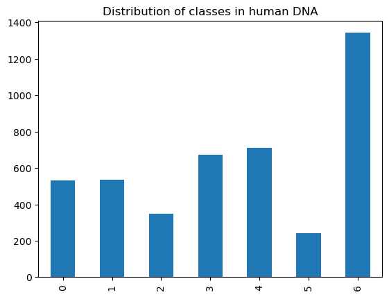
human_dna['class'].value_counts().sort_index().plot.bar()
plt.title("Distribution of classes in human DNA")

Chimpanzee DNA

chimp_dna = pd.read_table('data/dna-sequence-dataset/chimpanzee.txt')
chimp_dna.head()

	-------------------- sequence ------------------- class
0	ATGCCCCAACTAAATACCGCCGTATGACCCACCATAATTACCCCCA...	4
1	ATGAACGAAAATCTATTCGCTTCATTCGCTGCCCCCACAATCCTAG...	4
2	ATGGCCTCGCGCTGGTGGCGGTGGCGACGCGGCTGCTCCTGGAGGC...	4
3	ATGGCCTCGCGCTGGTGGCGGTGGCGACGCGGCTGCTCCTGGAGGC...	4
4	ATGGGCAGCGCCAGCCCGGGTCTGAGCAGCGTGTCCCCCAGCCACC...	6

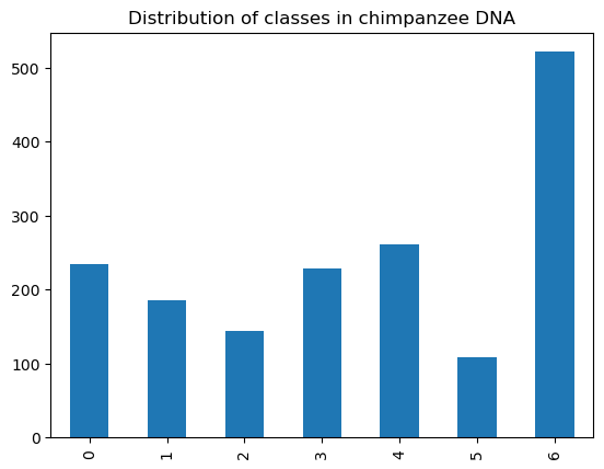
chimp_dna['class'].value_counts().sort_index().plot.bar()
plt.title("Distribution of classes in chimpanzee DNA")

Dog DNA

dog_dna = pd.read_table('data/dna-sequence-dataset/dog.txt')
dog_dna.head()

	-------------------- sequence ------------------- class
0	ATGCCACAGCTAGATACATCCACCTGATTTATTATAATCTTTTCAA...	4
1	ATGAACGAAAATCTATTCGCTTCTTTCGCTGCCCCCTCAATAATAG...	4
2	ATGGAAACACCCTTCTACGGCGATGAGGCGCTGAGCGGCCTGGGCG...	6
3	ATGTGCACTAAAATGGAACAGCCCTTCTACCACGACGACTCATACG...	6
4	ATGAGCCGGCAGCTAAACAGAAGCCAGAACTGCTCCTTCAGTGACG...	0

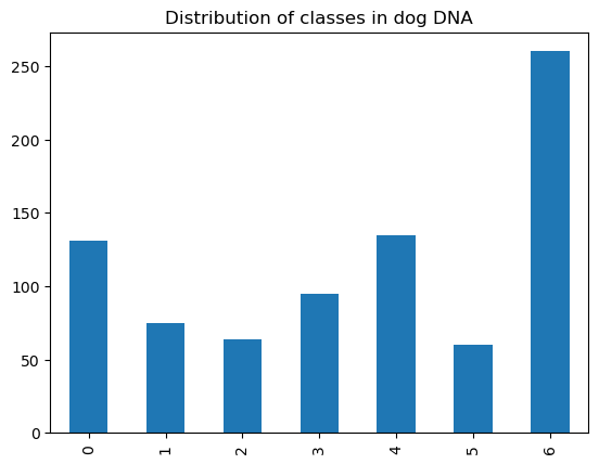
dog_dna['class'].value_counts().sort_index().plot.bar()
plt.title("Distribution of classes in dog DNA")

In the human DNA database, the 7 classes and their frequencies are as follows:
( 0 ) Protein-coupled receptors (count = 531)
( 1 ) Tyrosine kinase (count = 534)
( 2 ) Tyrosine phosphatase (count = 349)
( 3 ) Synthetase (count = 672)
( 4 ) Synthase (count = 711)
( 5 ) Ion channel (count = 240)
( 6 ) Transcription factor (count = 1343)

Collecting Hexamers

Now that our data is loaded, the next step is to convert a character sequence into k-mer words, specifically hexamers (k=6). The kmers() function will collect all possible k-mers (with overlap).

def kmers(seq, size=6):
    return [seq[x:x+size].upper() for x in range(len(seq) - size + 1)]

# our training data sequences are converted into hexamers
# the same process is then applied to different species

human_dna['words'] = human_dna.apply(lambda x: kmers(x['sequence']), axis=1)
human_dna = human_dna.drop('sequence', axis=1)

chimp_dna['words'] = chimp_dna.apply(lambda x: kmers(x['sequence']), axis=1)
chimp_dna = chimp_dna.drop('sequence', axis=1)

dog_dna['words'] = dog_dna.apply(lambda x: kmers(x['sequence']), axis=1)
dog_dna = dog_dna.drop('sequence', axis=1)

human_dna.head()

  class 					 words
0	4	[ATGCCC, TGCCCC, GCCCCA, CCCCAA, CCCAAC, CCAAC...
1	4	[ATGAAC, TGAACG, GAACGA, AACGAA, ACGAAA, CGAAA...
2	3	[ATGTGT, TGTGTG, GTGTGG, TGTGGC, GTGGCA, TGGCA...
3	3	[ATGTGT, TGTGTG, GTGTGG, TGTGGC, GTGGCA, TGGCA...
4	3	[ATGCAA, TGCAAC, GCAACA, CAACAG, AACAGC, ACAGC...

Now, for each gene, we need to convert the lists of hexamers into word phrases to create the bag-of-words model we want to establish. Additionally, we will define a variable y that will act as the target variable.

human_text = list(human_dna['words'])
for i in range(len(human_text)):
    human_text[i] = ' '.join(human_text[i])

chimp_text = list(chimp_dna['words'])
for i in range(len(chimp_text)):
    chimp_text[i] = ' '.join(chimp_text[i])

dog_text = list(dog_dna['words'])
for i in range(len(dog_text)):
    dog_text[i] = ' '.join(dog_text[i])

# the labels are separated
y_human = human_dna.iloc[:, 0].values
y_chimp = chimp_dna.iloc[:, 0].values
y_dog = dog_dna.iloc[:, 0].values

y_human

Thus, the target variable contains an array of classes.

Next, we will use the bag-of-words model using CountVectorizer(), which is equivalent to k-mer counting. By default, we will use n-grams (subsequences of n elements), and we will convert our k-mers into numerical vectors of uniform length, representing the count of each k-mer.

cv = CountVectorizer(ngram_range=(4,4))
X_human = cv.fit_transform(human_text)
X_chimp = cv.transform(chimp_text)
X_dog = cv.transform(dog_text)

print("For humans, we have {} genes converted into uniform-length vectors for counting 4-gram hexamers.".format(X_human.shape[0]))
print("For chimpanzees, we have {} genes converted into uniform-length vectors for counting 4-gram hexamers.".format(X_chimp.shape[0]))
print("For dogs, we have {} genes converted into uniform-length vectors for counting 4-gram hexamers.".format(X_dog.shape[0]))

For humans, we have 4380 genes converted into uniform-length vectors for counting 4-gram hexamers.
For chimpanzees, we have 1682 genes converted into uniform-length vectors for counting 4-gram hexamers.
For dogs, we have 820 genes converted into uniform-length vectors for counting 4-gram hexamers.

Now that we know how to transform DNA sequences into numerical vectors of uniform length for k-mer and n-gram counting, we can go further and design a classification model that predicts the function of a DNA sequence based on that sequence.

We will only use human DNA to train the model, with 20% of human DNA used as test data. The goal is to have a generalized model that can be applied to DNA from different species (in this case, chimpanzees and dogs).

Therefore, we will build a naive Bayes multinomial classification model (naive because we assume strong independence of the hypotheses).

Note: To observe fluctuations and optimize the model, you can vary the parameters and build models with different n-gram sizes and different values for alpha.

# Split the human DNA data into training and test subsets
X_train, X_test, y_train, y_test = train_test_split(X_human, y_human, test_size=0.20, random_state=42)

Create a multinomial naive Bayes classifier. After several trials, the most optimized values for the n-gram size are 4, and alpha is 0.1.

classifier = MultinomialNB(alpha=0.1)
classifier.fit(X_train, y_train)

Predictions on Test Data

y_pred = classifier.predict(X_test)

We want to examine the model's performance, so we will focus on several metrics in detail: precision (correct predictions among all selected predictions), recall (correct predictions among all available predictions), accuracy, F1 score (harmonic mean of precision and recall), and the confusion matrix.

print("Confusion Matrix for predictions on human DNA sequences:\n")
print(pd.crosstab(pd.Series(y_test, name='Actual'), pd.Series(y_pred, name='Predicted')))

def metrics(y_test, y_predicted):
    accuracy = accuracy_score(y_test, y_predicted)
    precision = precision_score(y_test, y_predicted, average='weighted')
    recall = recall_score(y_test, y_predicted, average='weighted')
    f1 = f1_score(y_test, y_predicted, average='weighted')
    return accuracy, precision, recall, f1

accuracy, precision, recall, f1 = metrics(y_test, y_pred)

print("\nAccuracy   = {} \nPrecision  = {} \nRecall     = {} \nF1 Score   = {}".format(accuracy, precision, recall, f1))

Confusion Matrix for predictions on human DNA sequences:

Predicted   0    1   2    3    4   5    6
Actual                                   
0          99    0   0    0    1   0    2
1           0  104   0    0    0   0    2
2           0    0  78    0    0   0    0
3           0    0   0  124    0   0    1
4           1    0   0    0  143   0    5
5           0    0   0    0    0  51    0
6           1    0   0    1    0   0  263

Accuracy   = 0.9840182648401826 
Precision  = 0.984290543482443 
Recall     = 0.9840182648401826 
F1 Score   = 0.9840270014702487

We tested the model on human DNA, which it learned from, so we logically obtained very good results. Now, let's put our model to the test by applying it to DNA from other species (chimpanzees and dogs).

First, chimpanzee DNA. We expect it to work well because chimpanzees and humans are biologically closely related, sharing a common ancestor.

y_pred_chimp = classifier.predict(X_chimp)

print("Confusion Matrix for predictions on chimpanzee DNA sequences:\n")
print(pd.crosstab(pd.Series(y_chimp, name='Actual'), pd.Series(y_pred_chimp, name='Predicted')))

accuracy, precision, recall, f1 = metrics(y_chimp, y_pred_chimp)

print("\nAccuracy   = {} \nPrecision  = {} \nRecall     = {} \nF1 Score   = {}".format(accuracy, precision, recall, f1))

Confusion Matrix for predictions on chimpanzee DNA sequences:

Predicted    0    1    2    3    4    5    6
Actual                                      
0          232    0    0    0    0    0    2
1            0  184    0    0    0    0    1
2            0    0  144    0    0    0    0
3            0    0    0  227    0    0    1
4            2    0    0    0  254    0    5
5            0    0    0    0    0  109    0
6            0    0    0    0    0    0  521

Accuracy   = 0.9934601664684899 
Precision  = 0.993551028649631 
Recall     = 0.9934601664684899 
F1 Score   = 0.993453334125236

Next, let's test the model on dog DNA. We expect lower performance.

y_pred_dog = classifier.predict(X_dog)

print("Confusion Matrix for predictions on dog DNA sequences:\n")
print(pd.crosstab(pd.Series(y_dog, name='Actual'), pd.Series(y_pred_dog, name='Predicted')))

accuracy, precision, recall, f1 = metrics(y_dog, y_pred_dog)

print("\nAccuracy   = {} \nPrecision  = {} \nRecall     = {} \nF1 Score   = {}".format(accuracy, precision, recall, f1))

Confusion Matrix for predictions on dog DNA sequences:

Predicted    0   1   2   3    4   5    6
Actual                                  
0          127   0   0   0    0   0    4
1            0  63   0   0    1   0   11
2            0   0  49   0    1   0   14
3            1   0   0  81    2   0   11
4            4   0   0   1  126   0    4
5            4   0   0   0    1  53    2
6            0   0   0   0    0   0  260

Accuracy   = 0.925609756097561 
Precision  = 0.9340667154775472 
Recall     = 0.925609756097561 
F1 Score   = 0.9251228556957126

Conclusion

As expected, the model produced very good results on human DNA and chimpanzee DNA, which share a common ancestor with humans. However, the model struggles more to classify DNA from species that are genetically distant from humans.