Photoreceptors detection and Biomimetism functions
Bio-robotic vision simulation
Project Details
- Category: Robotics & Embedded Systems
- Date: December 2022
- Language: MATLAB, Simulink
- GitHub: Project Repository
- Project Report
In collaboration with Ines Grellat-Sevilla, I worked on a project focused on mimicking drone vision and behavior using a bio-robot. We created an environment where the robot navigated between walls with gray-striped patterns of varying shades. By implementing Gaussian sensitivity functions and utilizing MATLAB and Simulink, we successfully simulated the photoreceptors' response to different shades of gray. Our project showcased the potential of biomimicry and advanced computational tools in replicating natural sensory systems.
The Project
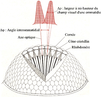
Context
The project is based on a fly’s vision and behavior, through biomimicry. The general purpose is to create a bio-robot imitating the patterns and movements of a fly. Our specific approach focuses on the interaction between the photoreceptors of the fly’s eye and the perceived environment.
The point of the project is for the robot to move between two walls composed of stripes of different shades of gray. To achieve this project, we will assume that our fly only moves in a single direction and we want to simulate its vision considering the Gaussian sensitivity of the photodiodes.
For simplicity’s sake, we are only going to consider two photoreceptors facing the same wall, and we are going to try to program the photoreceptors’ response.
Segmentation
Our project is composed of five major big steps:
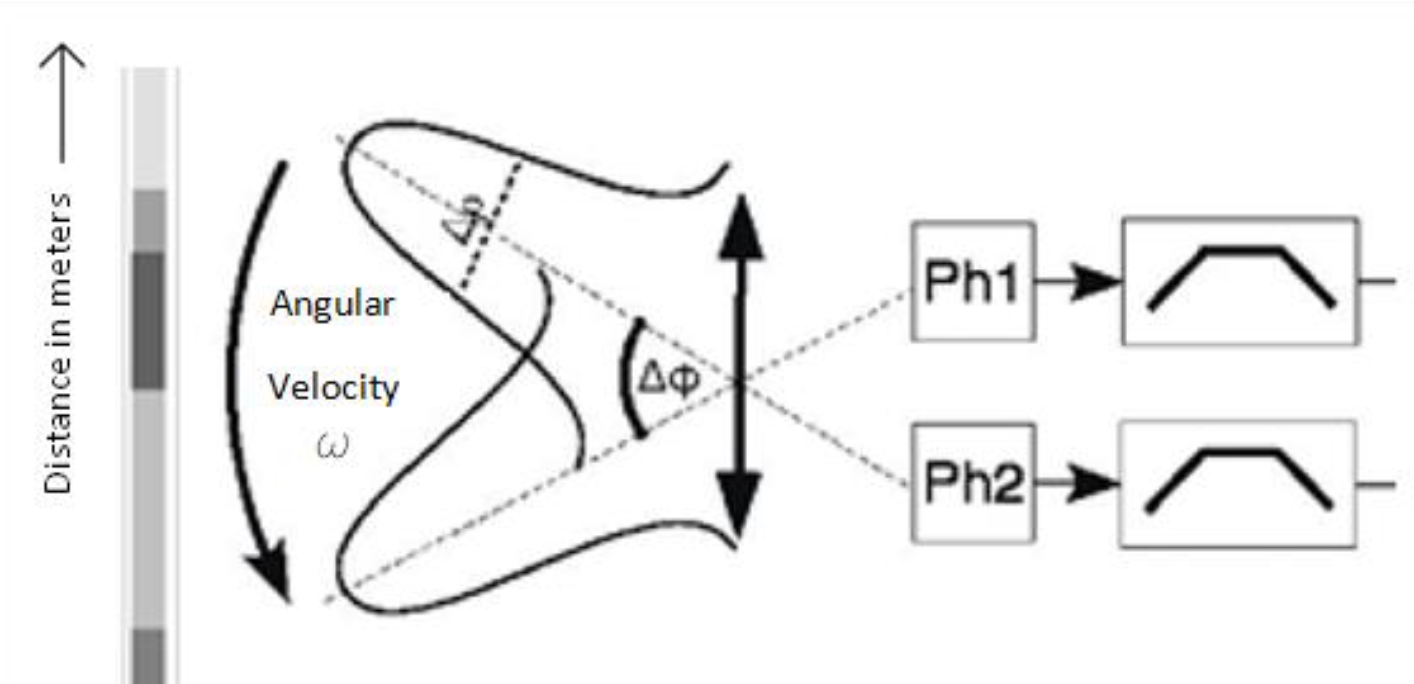
The photoreceptor has a Gaussian-shaped sensitivity, meaning that what is in the robot's peripheral vision won’t be as crucial in the calculation as what’s right in front of it.
The environment is a four meters long gray-striped wall, with distinct shades. The distinction between the shades will be the benchmarks in our calculus.
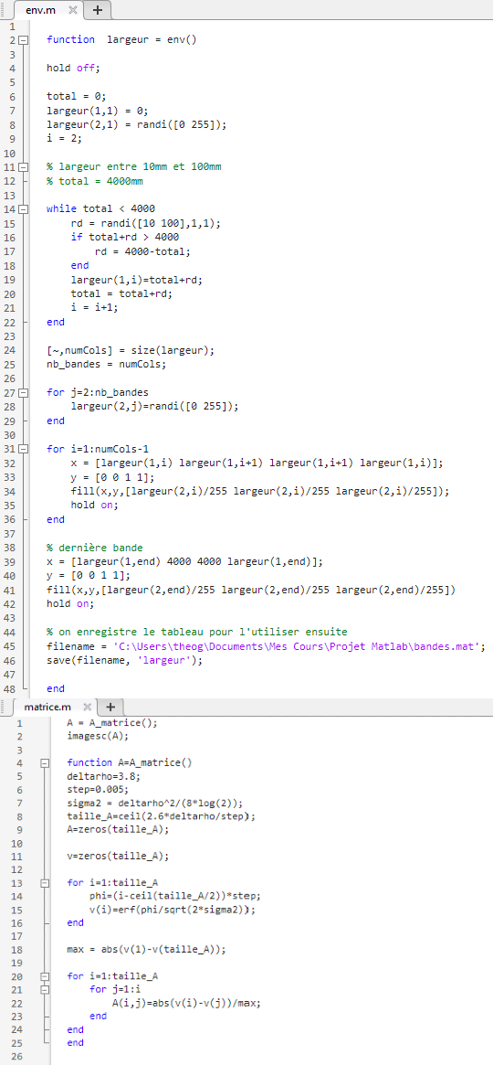
Environment
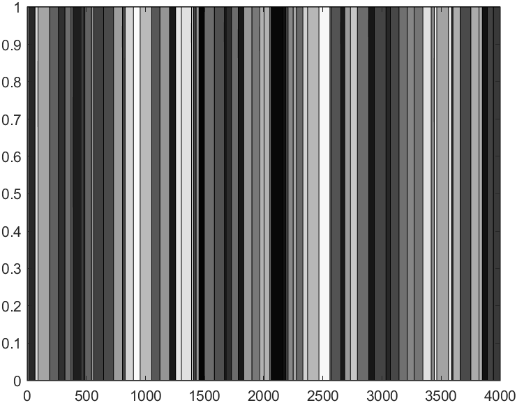
The first step in our biomimicry project is to model the environment in which our fly will evolve. The model will only contain one dimension (the x-axis) for a 4-meter distance.
The key element in our model is that the environment is randomly generated by grey bands which length is included between 10mm and 100mm. The gray shade of every stripe is determined randomly, as well as the width thereof. Finally, the environment will have a resolution of Δx = 1mm.
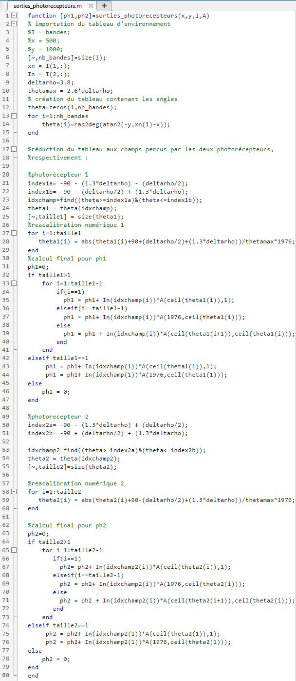
Look-up tables
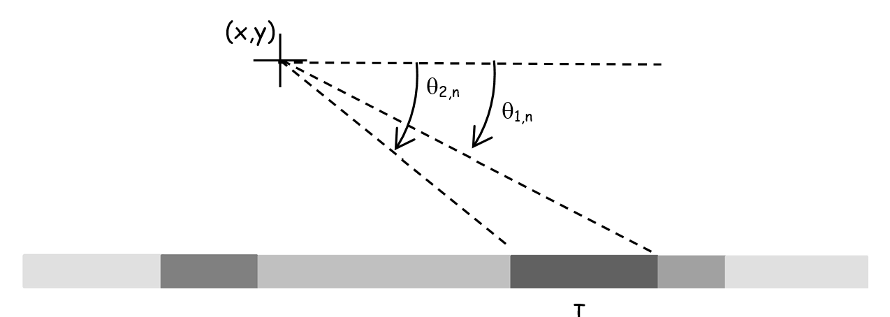
We just saw what the environment will look like, but our fly won't see it as clearly as we do. Indeed, it is the separation between two stripes that will determine the angle used later to calculate the sensitivity of the photoreceptor for the stripe considered. We will use a matrix to get what the photoreceptor perceives.
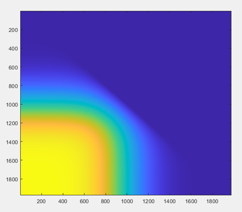
Basically, this matrix is used as a computational tool to simplify the integral of the Gaussian curve of photoreceptors as it represents a correspondence table thus allowing us to estimate the integral of the Gaussian sensitivity between two contrast transition angles. This matrix A will considerably reduce the execution time while modeling the photodiode outputs Ph1 and Ph2. Note that our matrix will be pre-calculated with a resolution δϕ = 0.005.
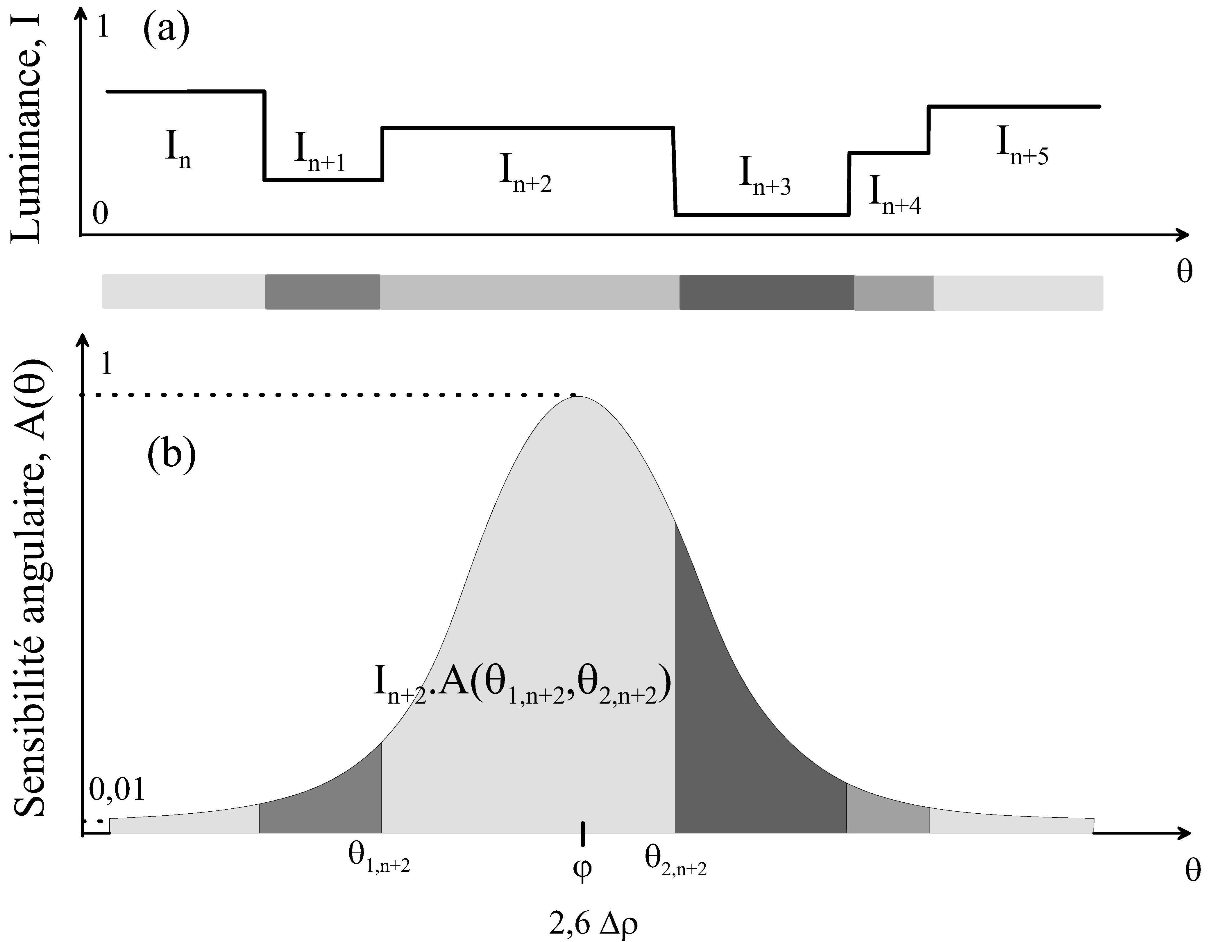
\((\varphi) = e^{-\frac{(\varphi - \varphi_{\text{max}})^2}{2\sigma^2}}\)
where:
We also know that a relation exists between Δρ and σ:
\(\Delta\rho = 2\sqrt{2\ln(2)}\sigma\)
At the end, the matrix contains every precalculated area of this Gaussian function, allowing us to determine exactly how much the photoreceptor is sensitive to a given stripe.
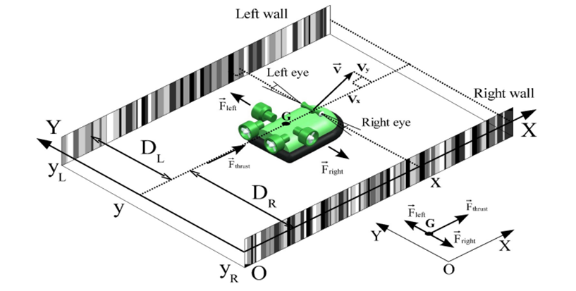
Simulating the photodetectors
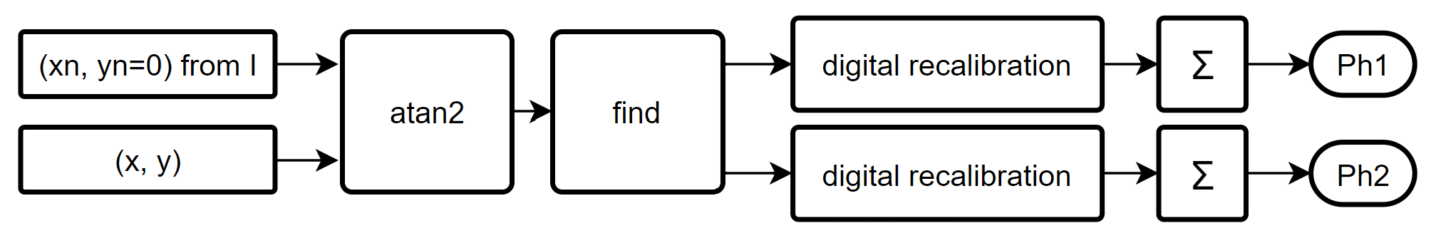
We successfully created an environment for our experiment. Now, we have to deduce from it the way the fly's photoreceptors will perceive the size and color of every band. The process we used is complex and can be explained by the organigram below.
Visual field of the photodetectors
The MatLab function "find" allowed us to select the angles that are in the visual field of each of the photoreceptors, knowing that they are separated by ±Δϕ/2 from the wall.
For Ph1:
\(-90^\circ - \frac{\Delta\phi}{2} - 1.3\Delta\rho \leq \theta_n \leq -90^\circ - \frac{\Delta\phi}{2} + 1.3\Delta\rho\)
For Ph2:
\(-90^\circ + \frac{\Delta\phi}{2} - 1.3\Delta\rho \leq \theta_n \leq -90^\circ + \frac{\Delta\phi}{2} + 1.3\Delta\rho\)
Digital recalibration
During this step, we want to ensure that 1 ≤ θₙ ≤ 1976 in order to then exploit the matrix A.
\( \text{recalibration} = \frac{\text{angle} - \text{angle\_min}}{\text{step}} \)
The matrix A
The matrix A is used to determine the output of each of the photoreceptors by summation:
\( \text{Ph} = \int I(\theta) \cdot A(\theta) \, d\theta \approx \sum_i I_n \cdot A(\theta_{1,n}, \theta_{2,n}) \)
Please note that while calculating the global perception of the photoreceptor, we use a discrete sum instead of an integral to simplify the computer's calculating process.
Results and photodetector outputs
Simulation parameters
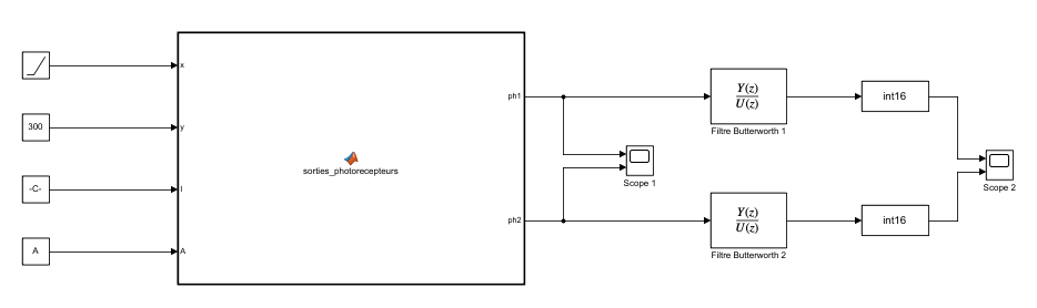
In order to correctly visualize the output of the two photodetectors, we used the Simulink software and we assumed that the fly moves parallel to the wall at 30 cm and a constant speed of 0.5 m/s, which is the role of the ramp block in our simulation.
Finally, we added a second-order digital bandpass filter [20 Hz; 116 Hz] and converted our data to 16 bits to simulate the analog-to-digital conversion of the microcontroller, with a temporal sampling frequency of 2 kHz.
Output visualization
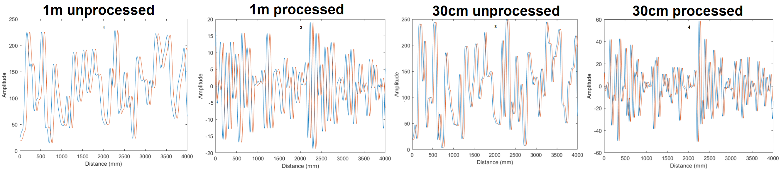
Interpretation
As we are moving from the wall, the two signals are shifting, which was expected. Moreover, it is clear that the results for the unprocessed output are smoother when we are farthest from the wall.
Conclusion
Our simulated environment is coherent and allows us to observe the evolution of the photoreceptor sensitivity. Our code is functional and could be implemented on a robot, proving the efficiency of biomimicry combined with new technologies.
Annexes